Indexing

---

In this note we will take a look at what are indexes, the different types of existing indices, and how they can be used in a given database. We will also take a look at B$^{\boldsymbol{+}}$-trees.

---

Indexing

In large datasets with multiple entries, it can become very expensive to perform lookups using only the primary key. The solution for this is indexing: just like a book catalog in a library, an index catalogs entries according to an attribute or set of attributes. This attribute is called the search-key of the index.

An index file will consist of several index entries, which have the following aspect:

Fig.1: Index entry example

info

Index files are typically much shorter than the original file containing the data

There are two types of indexes (which we will go into deeper detail):

• Ordered Indices: search keys are stored in sorted order
• Hash Indices: search keys are distributed across buckets using hash functions

Ordered Indices

In ordered indices, index entries are stored in a file sorted by their search key value. We can then specify two types of ordered indices:

• Clustered Index: The order in this index specifies the sequential order in the data file
  • Usually (but not always) the search key of this index corresponds to the primary key
• Non-Clustered Index: An index which specifies an order different from the one in the file

Dense Index File

In a dense index, there exists a index entry for every search-key value in the file.

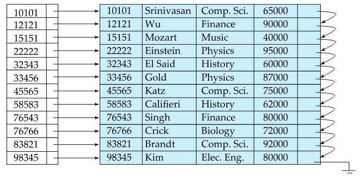
Fig.2: Dense index example (index on id)

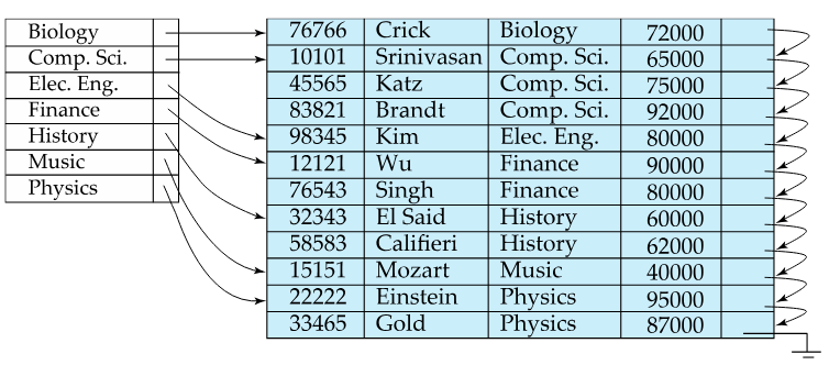
Fig.3: Another example of a dense index, this time on dept. name

Sparse Index Files

In sparse index files, the opposite happens: there is only index entries for some search-key values. This is only applicable when the records are sequentially ordered on the search-key:

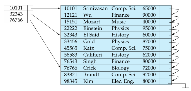
Fig.4: Sparse index example

Dense vs Sparse Indices

The main tradeoff that has to be considered when comparing dense and sparse indexes is choosing between speed and size:

• Dense indexes are faster than sparse indexes at doing lookups of entries
• Sparse indexes occupy less space than dense indexes

Clustered vs Non-Clustered Indices

Now that we have seen the differences between dense and sparse indices, we can correlate take the following conclusions:

• Non-Clustered Indices have to be dense indices. This is because sparse indices must be ordered on their particular search-key, and the records are only sequentially ordered according to clustered indices
• Sequential scan using a clustered index is efficient, as opposed to a non-clustered index where doing this is inefficient

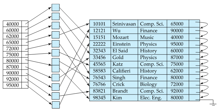
Fig.5: Non-clustered index example

B$^{\textbf{+}}$-Tree Indices

Ordered indices can also be of the B$^{\textbf{+}}$-tree format. A B$^{\textbf{+}}$-tree follows the following properties:

• All paths from root to leaf are the same length
• Each node that is not a root or a leaf has between $\lceil \dfrac{n}{2} \rceil$ and $\lceil n \rceil$ children
• A leaf node has between $\lceil \dfrac{n - 1}{2} \rceil$ and $\lceil n - 1 \rceil$ values
• Special cases:
  • If the root is not a leaf, it has at least two children
  • If the root is the leaf (there are no other values nodes in the tree), it can have between $0$ and $n - 1$ values

info

$n$ is a predefined value, that establishes how large is each B$^{\textbf{+}}$-Tree node

Up next is an example of a B$^{\textbf{+}}$-tree:

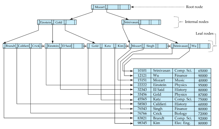
Fig.6: B$^{\textbf{+}}$-Tree example

B$^{\textbf{+}}$-Tree Node Structure

A typical node of a B$^{\textbf{+}}$-Tree is composed by several of the following two elements:

• Search-key values (K$_{i}$)
• Pointers to other nodes (children) or pointers to records (P$_{i}$)

These elements are then intercalated, and a node will have the following structure:

Fig.7: B$^{\textbf{+}}$-Tree node structure

Also, the search-keys in a node are structured, i.e.:

• K$_{1}$ < K$_{2}$ ... K$_{n - 2}$ < K$_{n - 1}$

Leaf Nodes

Each leaf node has the following properties:

• P$_{i}$ ($i \neq n$) points to a record/bucket of records with search-key value equal to K$_{i}$
• Pointer P$_{n}$ points to the next leaf node (according to search-key order)
• If L$_{i}$ and L$_{j}$ are both leaf nodes, with $i < j$, then all L$_{i}$'s search-key values are $\le$ than L$_{j}$'s search-key values

Non-leaf Nodes

A good way to think about non-leaf nodes (root and internal nodes) is that they form a multilevel sparse index on leaf nodes.

Considering the example above of a node structure:

• All the search keys for which the pointer P$_{1}$ points are $\lt$ K$_{1}$
• All the search keys pointed by P$_{i}$, with $2 \le i \le n - 1$ are $\lt$ K$_{i}$ and $\ge$ K$_{i - 1}$
• All the search keys pointed by P$_{n}$ are $\ge$ K$_{n - 1}$

Up next is an example of a B$^{\textbf{+}}$-Tree following these rules:

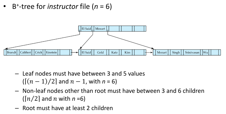
Fig.8: B$^{\textbf{+}}$-Tree structure example with n = 6

Observations about B$^{\textbf{+}}$-Trees

• Since nodes connect to each other, logically "close" nodes do not need to be physically stored next to each other (facilitates storing)
• B$^{\textbf{+}}$-Trees contain few levels, since each level exponentially stores more and more values (in relation to n):
  • Level below root stores $2 \cdot \lceil \dfrac{n}{2} \rceil$ values
  • Level below that stores $2 \cdot \lceil \dfrac{n}{2} \rceil \cdot \lceil \dfrac{n}{2} \rceil$ values
  • Etc...
• If there are 𝐾 search-key values in the file, the tree height is no more than $\lceil \log_{\lceil n / 2 \rceil}(K) \rceil$thus searches can be conducted efficiently. ^ad65a1
• Because the index can be restructured in logarithmic time, insertions and deletions are efficient

Queries on B$^{\textbf{+}}$-Trees

Algorithm

The algorithm to find a value $V$ in a B$^{\textbf{+}}$-Tree is the following:

• Starting on the root node:

  1. If there is $K_{i}$ such that $K_{i} = V$, then follow pointer $P_{i+1}$
  2. If there is $K_{i}$ such that $V < K_{i}$, then follow pointer $K_{i}$
  3. If no $K_{i}$ found that satisfies the last two properties, then follow the last pointer

• Repeat this until a leaf node is reached

• Once a leaf node is reached:

  1. If there is $K_{i}$ such that $V = K_{i}$, then follow $P_{i}$
  2. If there is no such $K_{i}$, that means that $V$ doesn't exist in this index

Range Queries

To perform a range query (i.e., find all values $V$ that satisfy $V_{\textbf{min}} \le V \le V_{\textbf{max}}$), this is the algorithm:

1. Perform a normal query on value $V_{\textbf{min}}$, using the algorithm above.
2. After finding $V_{\textbf{min}}$, go through every value followed by it (using pointers to the next leaf node)
3. Retrieve values from every pointer $P_{i}$ such that $V_{\textbf{min}} \le K \le V_{\textbf{max}}$
4. Stop upon finding the first $K_{i}$ such that $V_{\textbf{max}} < K_{i}$, or go until the end

Query Performance

If we look closely at the algorithm used for queries in B$^{\textbf{+}}$-trees, we can clearly see that query time is directly affected by the height of tree* that, like we saw here, is equal to $\lceil \log_{\lceil n / 2 \rceil}(K) \rceil$. In a real world implementation of a B$^{\textbf{+}}$-tree, $n$ is typically around 100; with $K = 1,000,000$, we have:

• At most $log_{50} 1,000,000$ nodes are accessed, which corresponds to only 4 nodes
• In a balanced binary tree, we wold have to traverse about 20 nodes

Updates on B$^{\textbf{+}}$-Trees

We will take a look at how to insert and delete values from B$^{\textbf{+}}$-trees.

Insertion

To insert a value into a B$^{\textbf{+}}$-tree, we assume that the record was already added to the file. Then we consider:

• $P_{r}$ to be the pointer to the record
• $K_{r}$ to be the search-key of that record

We then find the lead node where that record would be (with the current tree). If there is space in that leaf, we insert the pair $(K_{r}\ , \ P_{r})$ into that leaf node. If not, we will need to split the leaf node:

Splitting a Leaf Node

The algorithm for inserting a value into a full leaf node is the following:

1. Take the $n$ pairs (search-key, pointer) of the leaf node where we would insert $(K_{r}\ , \ P_{r})$, plus the pair $(K_{r}\ , \ P_{r})$, and place the first $\lceil \dfrac{n}{2} \rceil$ nodes in the original node, and the rest in a new node
2. Let the new node be $p$ and $k$ the least key value in $p$. Insert $(k\ ,\ p)$ into the parent of the node being split
3. If the parent node, split it too (and do this if its parent is full, etc.)

Up next are two examples of this:

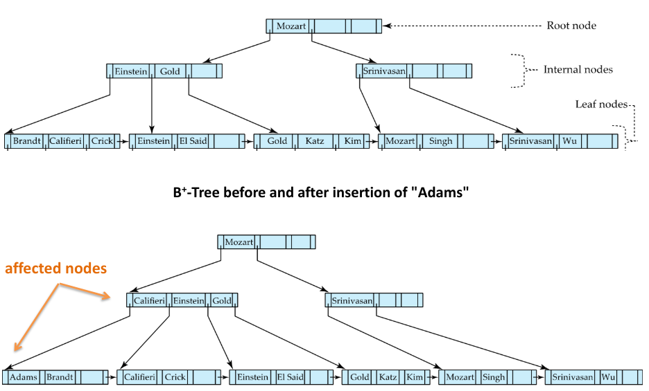
Fig.9: Example of a B$^{\textbf{+}}$-tree insertion

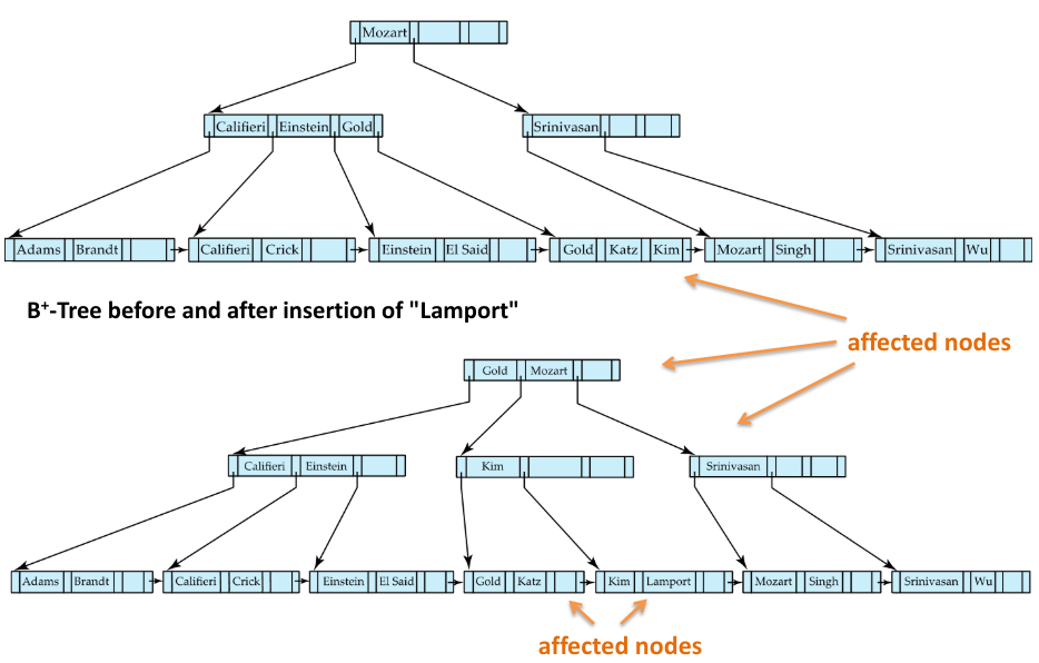
Fig.10: Another example of a B$^{\textbf{+}}$-tree insertion

Deletion

Just like in inserting a value into a B$^{\textbf{+}}$-tree, when deleting a value we assume we have already deleted the value; we then evaluate if the node has too few elements: if it does not, we leave it as is; if it does, we will have to perform some merges.

Let:

• $P_{r}$ be the pointer of the entry to be removed
• $K_{r}$ to be the search-key of the entry to be removed

If the node has too few entries, and if the node itself and its sibling fit into a single node, then we can merge the two nodes:

1. Insert all the values into a single node (the one on the left) and delete the other node (the one on the right)
2. In the parent node of the deleted node, delete the pair $(K_{i - 1}\ ,\ P_{i})$, being $P_{i}$ the pointer that pointed to the deleted node
3. If the parent node also has too few entries, repeat the previous two steps recursively

Otherwise, if the node has too few entries due to the removal, but the entries in the node and a sibling do not fit into a single node, then redistribute pointers:

• Redistribute the pointers between the node and a sibling such that both have more than the minimum number of entries
• Update the corresponding search-key value in the parent of the node

The following three images show examples of deletions in B$^{\textbf{+}}$-trees:

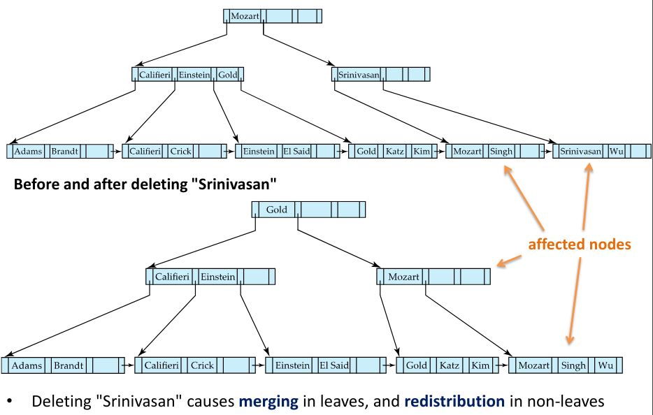
Fig.11: Example of a deletion in a B$^{\textbf{+}}$-tree

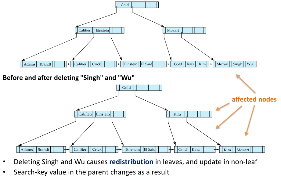
Fig.12: Example of a deletion in a B$^{\textbf{+}}$-tree

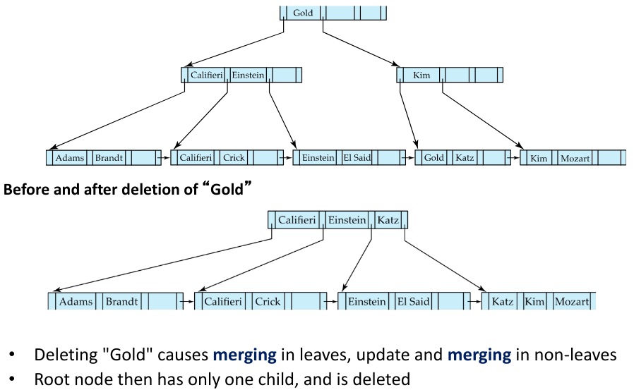
Fig.13: Example of a deletion in a B$^{\textbf{+}}$-tree

Update Cost

As we saw in the previous two chapters, in both insertions and deletions the total number of operations (splitting/merging nodes) it has to be done to complete these updates is directly related to the height of the tree. Therefore, we can conclude that, in the worst case, an update to a B$^{\textbf{+}}$-tree has the complexity:

• $O(\log_{\lceil n / 2 \rceil}(K))$

However, this is in the worst case. In practice, splits/merges are rare, and inserts and deletes are very efficient.

B$^{\textbf{+}}$-tree File Organization

A B$^{\textbf{+}}$-tree with file organization has exactly the same structure has the B$^{\textbf{+}}$-tree we saw in the previous chapters, with the exception that leafs hold the records themselves, not pointers to the records. This has the advantage of helping keep data clustered; however, because size restrictions are still the same, and records occupy more space than pointers, leaf nodes can hold less records when compared with a B$^{\textbf{+}}$-tree with pointers.

info

Insertion and deletion are handled in the same way as a B$^{\textbf{+}}$-tree index

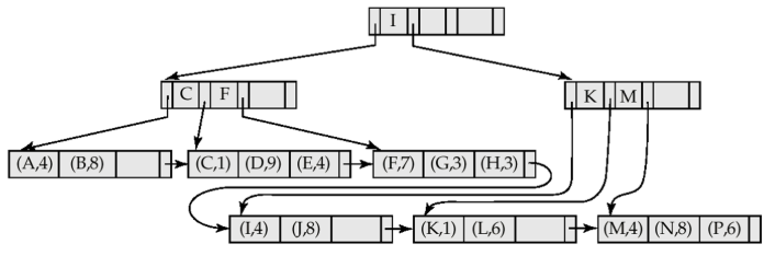
Fig.14: Example of a B$^{\textbf{+}}$-tree file organization